27 Week 14 Lab
In lab we’ll go through
Some practice with PCA using the semester survey results
Some practice with GLMs using the semester survey results
There are a number of functions you could use in R to do principal components analysis. We will use the ‘prcomp’ function, but there is a very closely related function called ‘princomp’ as well as a function called ‘principal’ which is in the ‘psych’ package.
readings<-read.csv("~/Dropbox/Biometry/Week 14 Multivariate analyses and Review/Week 14 Lab/Readings 2024.csv",header=T)

missing<-is.na(readings$Useful)|is.na(readings$Difficult)|is.na(readings$Interesting)

Useful<-aggregate(readings$Useful[!missing], by=list(Index=readings$Index[!missing]),FUN=mean)$x

Difficult<-aggregate(readings$Difficult[!missing], by=list(Index=readings$Index[!missing]),FUN=mean)$x

Interesting<-aggregate(readings$Interesting[!missing], by=list(Index=readings$Index[!missing]),FUN=mean)$x

Length.means.readings<-aggregate(readings$Length[!missing], by=list(Index=readings$Index[!missing]),FUN=mean)$x

pca.result<-prcomp(~Useful+Interesting+Difficult,retx=T)
Before printing out the result, let’s make sure everyone understands what I was doing with the aggregate commands, and how the ‘prcomp’ function input works.
To print out a summary of the PCA, we use
## Importance of components:
##                           PC1    PC2    PC3
## Standard deviation     0.9046 0.7529 0.4896
## Proportion of Variance 0.5036 0.3489 0.1475
## Cumulative Proportion  0.5036 0.8525 1.0000
We see that PCA1 is associated with over 50% of the variation in responses. So, what is PCA1?
##                      PC1       PC2        PC3
## Useful      -0.006816199 0.4357315  0.9000509
## Interesting  0.843748274 0.4855820 -0.2286896
## Difficult   -0.536695807 0.7578576 -0.3709576
PCA1 is an axis which describes papers that are more Interesting and less Difficult, with a tiny weight towards papers that are less Useful. In other words, a large positive PCA1 score would be associated with an interesting paper that was easy to read. Note that the principal components denote an axis, but the direction is arbitrary. Since no direction is implied by the sign, we do not interpret this as saying that most papers were interesting and easy. Instead we would say that the papers largely fall along a common axis in which Interesting/Easy to read papers are at one end, and Boring/Difficult to read papers are at the other end. (For now I am ignoring the smaller influence of Useful on PCA1.)
We can visualize this using the function ‘biplot’
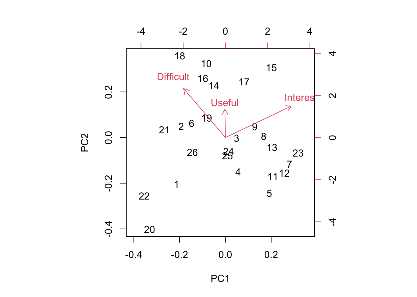
Biplots take some getting used to, and when they have many more dimensions, they become increasingly difficult to interpret. However, papers high on PC1 are generally Interesting and Easy to read and papers low on PC1 are generally Boring and more Difficult to read. Papers high on PC2 are generally Useful, Difficult, and Interesting all at the same time and papers low on PC2 are generally less Useful and less Difficult to read and less Interesting. It’s worth noting that there is a nice spread of papers in this bi-plot, so at least along these two axes, there were no real outliers. Also, keep in mind that since the PCA is picking up relative differences, it is not possible for all papers to end up in one corner of the plot. While of course we would want all papers to be highly Interesting and highly Useful, even if all papers ranked high on both measures overall, the PCA will identify axes of differences so there will always be some that show up as “relatively less Interesting” - does this make sense?
Which papers were positive on PC2 and also positive on PC1? These are papers that were more generally more Useful and Interesting than the average.
## [1] "Siddhartha, R. D., E. B. Fowlkes, and B. Hoadley. 1989. Risk analysis of the space shuttle: Pre-challenger prediction of failure. Journal of the American Statistical Association 84(408): 945-957."## [1] "Altman, N., and M. Krzywinski. 2015. Split plot design. Nature Methods 12(3): 165-166. (optional)"I totally agree on the Siddhartha paper! This paper is regularly rated highly. Altman and Krzywinski (1015) also fell into this category, though on the basis of only three ratings. This suggests everyone else should go back and read this paper!
You can play around with this yourself and see why I added the [1] at the end. When I pull out the rows with the Index identified by the PCA, I get the list of all entries (since we had >1 team rating the papers) and so I only print the first one.
Which paper fell out along the Difficult axis?
## [1] "Hurlbert, S. H. 1984. Pseudoreplication and the design of ecological field experiments. Ecological Monographs 54(2): 187-211."Hurlbert’s famous pseudoreplication paper.
Usually Bolker holds this honor! Bolker is often rated as difficult. I keep this chapter around because his thinking is so “spot on” and the material in his book will serve you well if you continue on doing quantitative modelling.
The real quadrant that I investigate closely are papers that are considered Difficult but not all that Useful. Through this PCA exeercise, I have eliminated papers consistently falling into this corner. Let’s see what 16 is…
## [1] "Krzywinski, M., N. Altman, and P. Blainey. 2014. Nested designs. Nature Methods 11(10): 977-978. (optional)"I’m surprised to see Krzywinski here, as the Points of Significance papers are so short and I think quite well written. I think this probably means we just need to spend a bit of time going over this one next year.
One thing to keep in mind is that a PCA identifies variation in the dataset. It’s worth putting these numbers in context of the overall means.
## [1] 3.969734## [1] 2.637065## [1] 3.215133So the average reading scored pretty high for being Useful and Interesting and was rated below average for Difficulty, so on the whole, I’m fairly pleased with these ratings.
You might be interested in how these ratings have changed over time (I was!). Let’s start with the readings.
library(readxl)
Biometry_change <- read_excel("_data/Biometry_change.xlsx")
fitR_U<-summary(lm(Biometry_change$R_U_mean~Biometry_change$Year))
fitR_U
##
## Call:
## lm(formula = Biometry_change$R_U_mean ~ Biometry_change$Year)
##
## Residuals:
## Min 1Q Median 3Q Max
## -0.36439 -0.26399 0.06366 0.16202 0.38224
##
## Coefficients:
## Estimate Std. Error t value Pr(>|t|)
## (Intercept) -85.55852 51.82955 -1.651 0.150
## Biometry_change$Year 0.04416 0.02569 1.719 0.136
##
## Residual standard error: 0.2946 on 6 degrees of freedom
## Multiple R-squared: 0.33, Adjusted R-squared: 0.2183
## F-statistic: 2.955 on 1 and 6 DF, p-value: 0.1364plot(Biometry_change$Year,Biometry_change$R_U_mean,pch=15,xlab="Year",ylab="Mean Response (out of 5)",cex=2,ylim=c(1.5,4.5),main="Useful (black), Difficult (red), Interesting (green)")
for (i in 1:9)
{
segments(x0=Biometry_change$Year[i], x1=Biometry_change$Year[i], y0=Biometry_change$R_U_mean[i]-2*Biometry_change$R_U_se[i],y1=Biometry_change$R_U_mean[i]+2*Biometry_change$R_U_se[i])
}
fitR_D<-summary(lm(Biometry_change$R_D_mean~Biometry_change$Year))
fitR_D##
## Call:
## lm(formula = Biometry_change$R_D_mean ~ Biometry_change$Year)
##
## Residuals:
## Min 1Q Median 3Q Max
## -0.29893 -0.12886 0.03503 0.12404 0.31271
##
## Coefficients:
## Estimate Std. Error t value Pr(>|t|)
## (Intercept) -39.63356 39.88751 -0.994 0.359
## Biometry_change$Year 0.02076 0.01977 1.050 0.334
##
## Residual standard error: 0.2267 on 6 degrees of freedom
## Multiple R-squared: 0.1553, Adjusted R-squared: 0.01454
## F-statistic: 1.103 on 1 and 6 DF, p-value: 0.334points(Biometry_change$Year,Biometry_change$R_D_mean,pch=15,xlab="Year",ylab="Mean Difficult",cex=2,col=2)
for (i in 1:9)
{
segments(x0=Biometry_change$Year[i], x1=Biometry_change$Year[i], y0=Biometry_change$R_D_mean[i]-2*Biometry_change$R_D_se[i],y1=Biometry_change$R_D_mean[i]+2*Biometry_change$R_D_se[i],col=2)
}
fitR_I<-summary(lm(Biometry_change$R_I_mean~Biometry_change$Year))
fitR_I##
## Call:
## lm(formula = Biometry_change$R_I_mean ~ Biometry_change$Year)
##
## Residuals:
## Min 1Q Median 3Q Max
## -0.19171 -0.11413 -0.03823 0.12481 0.21891
##
## Coefficients:
## Estimate Std. Error t value Pr(>|t|)
## (Intercept) -72.68056 29.30218 -2.480 0.0478 *
## Biometry_change$Year 0.03766 0.01452 2.593 0.0410 *
## ---
## Signif. codes: 0 '***' 0.001 '**' 0.01 '*' 0.05 '.' 0.1 ' ' 1
##
## Residual standard error: 0.1665 on 6 degrees of freedom
## Multiple R-squared: 0.5284, Adjusted R-squared: 0.4498
## F-statistic: 6.724 on 1 and 6 DF, p-value: 0.04105points(Biometry_change$Year,Biometry_change$R_I_mean,pch=15,xlab="Year",ylab="Mean Difficult",cex=2,col=3)
for (i in 1:9)
{
segments(x0=Biometry_change$Year[i], x1=Biometry_change$Year[i], y0=Biometry_change$R_I_mean[i]-2*Biometry_change$R_I_se[i],y1=Biometry_change$R_I_mean[i]+2*Biometry_change$R_I_se[i],col=3)
}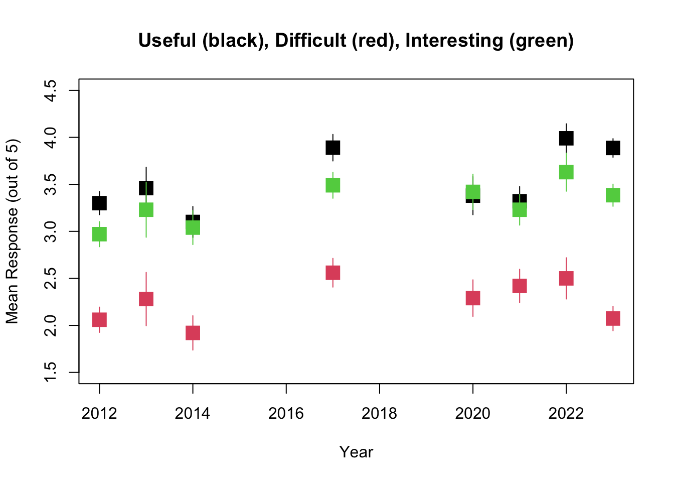
So it looks like while the overall trend is towards readings that are more Interesting, more Difficult, and more Useful, the only one of these that is statistically significant is the trend towards more Interesting.
The problem sets show exactly the same trends, with no significant changes in Useful or Difficult but a significant trend towards ore Interesting problem sets.
PS<-read.csv("~/Dropbox/Biometry/Week 14 Multivariate analyses and Review/Week 14 Lab/ProblemSets 2024.csv",header=T)

missing<-is.na(PS$Useful)|is.na(PS$Difficult)|is.na(PS$Interesting)

Useful.means.PS<-aggregate(PS$Useful[!missing], by=list(Index=PS$Week[!missing]),FUN=mean)$x

Difficult.means.PS<-aggregate(PS$Difficult[!missing], by=list(Week=PS$Week[!missing]),FUN=mean)$x

Interesting.means.PS<-aggregate(PS$Interesting[!missing], by=list(Week=PS$Week[!missing]),FUN=mean)$x

pca.result<-prcomp(~Useful.means.PS+Interesting.means.PS+Difficult.means.PS,data=PS,retx=T)
Notice that it has simply labeled them in order, so 7=Week #9 PS, 8=Week #10 PS, 9=Week #11 PS, 10=Week #12 PS, and 11=Week #13 PS.
To print out a summary of the PCA, we use
## Importance of components:
##                           PC1    PC2    PC3
## Standard deviation     0.8875 0.5784 0.1882
## Proportion of Variance 0.6804 0.2890 0.0306
## Cumulative Proportion  0.6804 0.9694 1.0000
We see that for the problem sets, PC1 is more dominant (89% of the variation). So, what is PCA1?
##                             PC1        PC2        PC3
## Useful.means.PS       0.6594159 -0.2519202 -0.7083127
## Interesting.means.PS  0.5391668 -0.4981108  0.6791059
## Difficult.means.PS   -0.5238987 -0.8297119 -0.1926352
PC1 combines all three factors with the largest component being focused on “Useful”, and the axis divides problem sets judged Useful/Interesting/Easy and those that are Less Useful/Less Interesting/Easy. (Reminder: the signs of the PCs is arbitrary, so the signs on the rotation could have all be flipped.) Looking across all the PC axes, we want papers that are positive on PC1 and negative on PC2. PC3 is a toss up, because that axis represents a trade-off between Useful and Interesting.
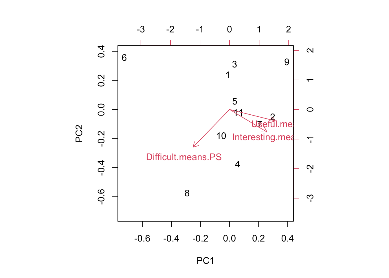
We can see that problem set 6 is the one that is really driving variation here! (As always) If we were to eliminate week 6, the others are all varying primarily on PC2.
Again, looking at the means:
## [1] 4.043019## [1] 3.103084## [1] 3.281656Problem set 6 stands out as neither Useful or Interesting. sigh This one was actually written from scratch a couple years ago because students didn’t like the old Week 6 problem set either. Maybe it’s just the material?
How have things changed over time?
##
## Call:
## lm(formula = Biometry_change$PS_U_mean ~ Biometry_change$Year)
##
## Residuals:
##      Min       1Q   Median       3Q      Max
## -0.35934 -0.10749 -0.06325  0.05777  0.54458
##
## Coefficients:
##                       Estimate Std. Error t value Pr(>|t|)
## (Intercept)          -73.58452   49.66576  -1.482    0.189
## Biometry_change$Year   0.03848    0.02461   1.563    0.169
##
## Residual standard error: 0.2823 on 6 degrees of freedom
## Multiple R-squared:  0.2894, Adjusted R-squared:  0.171
## F-statistic: 2.444 on 1 and 6 DF, p-value: 0.169plot(Biometry_change$Year,Biometry_change$PS_U_mean,pch=15,xlab="Year",ylab="Mean Response (out of 5)",cex=2,ylim=c(2,5),main="Useful (black), Difficult (red), Interesting (green)")
for (i in 1:9)
{
segments(x0=Biometry_change$Year[i], x1=Biometry_change$Year[i], y0=Biometry_change$PS_U_mean[i]-2*Biometry_change$PS_U_se[i],y1=Biometry_change$PS_U_mean[i]+2*Biometry_change$PS_U_se[i])
}
fitPS_D<-summary(lm(Biometry_change$PS_D_mean~Biometry_change$Year))
fitPS_D##
## Call:
## lm(formula = Biometry_change$PS_D_mean ~ Biometry_change$Year)
##
## Residuals:
## Min 1Q Median 3Q Max
## -0.40591 -0.18510 0.03417 0.16826 0.38526
##
## Coefficients:
## Estimate Std. Error t value Pr(>|t|)
## (Intercept) -30.20979 50.25999 -0.601 0.570
## Biometry_change$Year 0.01655 0.02491 0.664 0.531
##
## Residual standard error: 0.2856 on 6 degrees of freedom
## Multiple R-squared: 0.0685, Adjusted R-squared: -0.08675
## F-statistic: 0.4412 on 1 and 6 DF, p-value: 0.5312points(Biometry_change$Year,Biometry_change$PS_D_mean,pch=15,xlab="Year",ylab="Mean Difficult",cex=2,col=2)
for (i in 1:9)
{
segments(x0=Biometry_change$Year[i], x1=Biometry_change$Year[i], y0=Biometry_change$PS_D_mean[i]-2*Biometry_change$PS_D_se[i],y1=Biometry_change$PS_D_mean[i]+2*Biometry_change$PS_D_se[i],col=2)
}
fitPS_I<-summary(lm(Biometry_change$PS_I_mean~Biometry_change$Year))
fitPS_I##
## Call:
## lm(formula = Biometry_change$PS_I_mean ~ Biometry_change$Year)
##
## Residuals:
## Min 1Q Median 3Q Max
## -0.44739 -0.17128 -0.01723 0.15788 0.44258
##
## Coefficients:
## Estimate Std. Error t value Pr(>|t|)
## (Intercept) -137.90978 55.40599 -2.489 0.0472 *
## Biometry_change$Year 0.07004 0.02746 2.551 0.0435 *
## ---
## Signif. codes: 0 '***' 0.001 '**' 0.01 '*' 0.05 '.' 0.1 ' ' 1
##
## Residual standard error: 0.3149 on 6 degrees of freedom
## Multiple R-squared: 0.5202, Adjusted R-squared: 0.4403
## F-statistic: 6.506 on 1 and 6 DF, p-value: 0.04345points(Biometry_change$Year,Biometry_change$PS_I_mean,pch=15,xlab="Year",ylab="Mean Difficult",cex=2,col=3)
for (i in 1:9)
{
segments(x0=Biometry_change$Year[i], x1=Biometry_change$Year[i], y0=Biometry_change$PS_I_mean[i]-2*Biometry_change$PS_I_se[i],y1=Biometry_change$PS_I_mean[i]+2*Biometry_change$PS_I_se[i],col=3)
}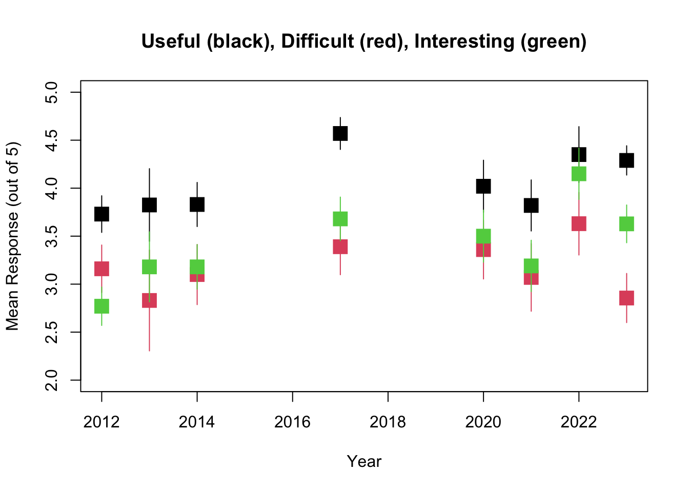
Interestingly, this is similar to the pattern seen for the Readings, with everything getting slightly more Useful and Difficult and Interesting but in this case none are statistically significant.
27.1 Missing at random - practice with GLMs
One of the things we can do with this dataset is to ask whether data were missing at random, since not all readings were given ratings.
missing<-is.na(readings$Useful)|is.na(readings$Difficult)|is.na(readings$Interesting)
Useful<-aggregate(readings$Useful[!missing], by=list(Index=readings$Index[!missing]),FUN=mean)$x

Difficult<-aggregate(readings$Difficult[!missing], by=list(Index=readings$Index[!missing]),FUN=mean)$x

Interesting<-aggregate(readings$Interesting[!missing], by=list(Index=readings$Index[!missing]),FUN=mean)$x

Length.means.readings<-aggregate(readings$Length[!missing], by=list(Index=readings$Index[!missing]),FUN=mean)$x
One could ask the question, are these data missing at random? In the problem set for Week #13, we completed the dataset using random imputation. In other words, we assumed that data were missing at random and we drew with replacement from the other values to replace missing datapoints. However, in this case, it seems likely that data are not missing at random. I suspect that papers were not evaluated because no one read them, and that something about the papers may predict whether the papers were read or not. We can answer this question by constructing a model for “missingness” which assumes that the probability of being evaluated is distributed as Binom(n,p) where p is the probability of being evaluated (and presumably, of having been read in the first place).
First, I need to go through the data and figure out how many times a paper was evaluated.
num.missing<-vector(length=max(readings$Index))
for (i in 1:max(readings$Index))
{
  num.missing.useful<-sum(as.numeric(is.na(readings$Useful[readings$Index==i])))
  num.missing.difficult<-sum(as.numeric(is.na(readings$Difficult[readings$Index==i])))
  num.missing.interesting<-sum(as.numeric(is.na(readings$Interesting[readings$Index==i])))
  max.missing<-max(num.missing.useful,num.missing.difficult,num.missing.interesting)
  num.missing[i]<-max.missing
}
num.missing<-num.missing[num.missing<8]
For simplicity, I am considering “evaluated” as evaluated for all three categories (Useful, Difficult, and Interesting). Also, there were a number of papers that not one single group read! Because no one read them, we have no ratings for Useful, Interesting, and Difficult and I have to take them out of the model (this is what I am doing in the last line of code above).
Now I use a Binomial GLM to model the probability of being evaluated as a function of Useful, Interesting, and Difficult (as rated by the other groups). Note that there were 8 groups total, so n=8.
fit<-glm(cbind(8-num.missing,num.missing)~Useful+Difficult+Interesting,family="binomial")
summary(fit)
##
## Call:
## glm(formula = cbind(8 - num.missing, num.missing) ~ Useful +
## Difficult + Interesting, family = "binomial")
##
## Deviance Residuals:
## Min 1Q Median 3Q Max
## -2.9189 -1.1350 0.1465 1.7006 2.7834
##
## Coefficients:
## Estimate Std. Error z value Pr(>|z|)
## (Intercept) 1.5058766 1.3869497 1.086 0.277591
## Useful -1.1667230 0.3477612 -3.355 0.000794 ***
## Difficult -0.0005351 0.2559736 -0.002 0.998332
## Interesting 1.2934373 0.2460047 5.258 1.46e-07 ***
## ---
## Signif. codes: 0 '***' 0.001 '**' 0.01 '*' 0.05 '.' 0.1 ' ' 1
##
## (Dispersion parameter for binomial family taken to be 1)
##
## Null deviance: 114.294 on 25 degrees of freedom
## Residual deviance: 66.559 on 22 degrees of freedom
## AIC: 110.84
##
## Number of Fisher Scoring iterations: 5Interestingly, papers more likely to be read were those that were relatively less Useful but they were Interesting. Perhaps they were read due to their perceived interestingness, but after the fact were found less useful than some of the other papers assigned.
We might suspect a high degree of multicollinearity among the predictors. We can use PCA to create new orthogonal covariates which (more efficiently) capture the variability in the survey results.
I will rerun the PCA for the readings.
## Importance of components:
##                           PC1    PC2    PC3
## Standard deviation     0.9046 0.7529 0.4896
## Proportion of Variance 0.5036 0.3489 0.1475
## Cumulative Proportion 0.5036 0.8525 1.0000## PC1 PC2 PC3
## Useful -0.006816199 0.4357315 0.9000509
## Interesting 0.843748274 0.4855820 -0.2286896
## Difficult -0.536695807 0.7578576 -0.3709576PCA1 captures about 50% of the variability, so we try using just PCA1 in our GLM.
##
## Call:
## glm(formula = cbind(8 - num.missing, num.missing) ~ pca.result$x[,
##     1], family = "binomial")
##
## Deviance Residuals:
##     Min       1Q   Median       3Q      Max
## -2.6797  -1.4587  -0.2318   1.6273   2.9878
##
## Coefficients:
##                   Estimate Std. Error z value Pr(>|z|)
## (Intercept)         1.0283     0.1761   5.839 5.26e-09 ***
## pca.result$x[, 1]   1.0823     0.2054   5.268 1.38e-07 ***
## ---
## Signif. codes:  0 '***' 0.001 '**' 0.01 '*' 0.05 '.' 0.1 ' ' 1
##
## (Dispersion parameter for binomial family taken to be 1)
##
##     Null deviance: 114.294  on 25  degrees of freedom
## Residual deviance:  80.705  on 24  degrees of freedom
## AIC: 120.98
##
## Number of Fisher Scoring iterations: 5
In this case, the collinearity is fairly weak and the model with just PC1 is actually worse (in the sense of having a higher AIC) than the original model with all three covariates included in the model separately.
Is there an effect of paper length to consider? After all, that’s probably the most salient feature of a paper when you first download it.
##
## Call:
## glm(formula = cbind(8 - num.missing, num.missing) ~ Length.means.readings,
##     family = "binomial")
##
## Deviance Residuals:
##     Min       1Q   Median       3Q      Max
## -3.9882  -1.4754   0.4313   2.3057   2.5694
##
## Coefficients:
##                       Estimate Std. Error z value Pr(>|z|)
## (Intercept)            0.58776    0.21927   2.681  0.00735 **
## Length.means.readings  0.02803    0.01784   1.571  0.11621
## ---
## Signif. codes:  0 '***' 0.001 '**' 0.01 '*' 0.05 '.' 0.1 ' ' 1
##
## (Dispersion parameter for binomial family taken to be 1)
##
##     Null deviance: 114.29  on 25  degrees of freedom
## Residual deviance: 111.17  on 24  degrees of freedom
## AIC: 151.45
##
## Number of Fisher Scoring iterations: 4
Longer papers are not more likely to be read than shorter papers.
27.2 Finally, a word about grades
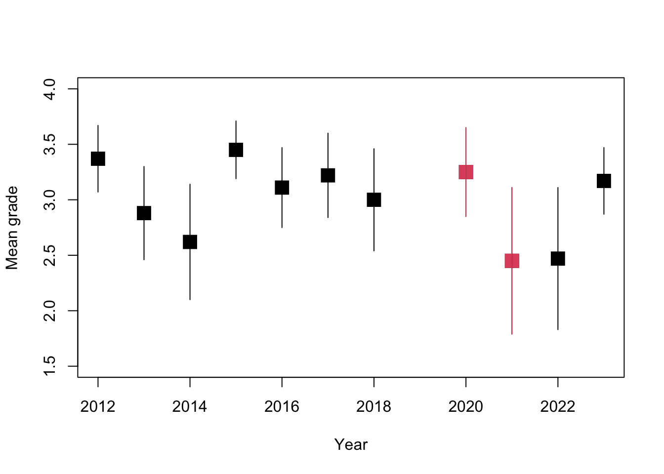
The question came up as to how grades have changed over time. Behold, the grade distribution over time (A=4, A-=3.67, B+=3.33, B=3, etc.).
year<-c(2012,2013,2014,2015,2016,2017,2018,2020,2021,2022,2023)
mean.grade<-c(3.37,2.88,2.62,3.45,3.11,3.22,3.00,3.25,2.45,2.47,3.17)
sem.grade<-c(0.15,0.21,0.26,0.13,0.18,0.19,0.23,0.20,0.33,0.32,0.15)
plot(year,mean.grade,pch=15,xlab="Year",ylab="Mean grade",cex=2,col=1,ylim=c(1.5,4))
points(year[c(8,9)],mean.grade[c(8,9)],pch=15,cex=2,col=2,ylim=c(1.5,4))
for (i in 1:length(mean.grade))
{
segments(x0=year[i], x1=year[i], y0=mean.grade[i]-2*sem.grade[i],y1=mean.grade[i]+2*sem.grade[i],col=1)
}
segments(x0=year[8], x1=year[8], y0=mean.grade[8]-2*sem.grade[8],y1=mean.grade[8]+2*sem.grade[8],col=2)
segments(x0=year[9], x1=year[9], y0=mean.grade[9]-2*sem.grade[9],y1=mean.grade[9]+2*sem.grade[9],col=2)